Python package exercise

Python package exercise#

In this exercises you will create your own ts_emergency package. You will first recreate the package covered in the packaging chapter and then modify the packaging module to be a namespace that contains two submodules.

Exercise 1#

The first job is to create the skeleton of the ts_emergency package. A link to the example data ed_ts_mth.csv is provided below.

Task

Create the directory, data and python module structure below. No code need be included at this stage.

ts_emergency
├── __init__.py
├── plotting.py
├── datasets.py
├── data
│   ├── syn_ts_ed_long.csv
│   ├── syn_ts_ed_wide.csv

Data files:

The dataset syn_ts_ed_long.csv contains data from 4 emergency departments in 2014. The data are stored in long (sometimes called tidy) format. You are provided with three columns: date (non unique date time formatted), hosp (int 1-4) and attends (int, daily number of attends at hosp \(i\))

The dataset syn_ts_wide.csv contains the same data in wide format. Each row now represents a unique date and each hospital ED has its own column.

The ed data is held in long format here
The ed data is held in wide format here

Hints:

Remember to think about where the local package needs to be stored relative to the code that is going to use it.
You can choose to use either the long format or short format data for this exercise. For basic plotting is is often easier to use a wide format.

Exercise 2:#

Task:

Add appropraite __version__ and __author__ attributes to __init__.py
Check these work by importing your package and printing the relevant attributes.

Hints:

These should be of type str

# your code testing your package here ...

# example solution

import ts_emergency as tse
print(tse.__version__)
print(tse.__author__)

0.1.0
Tom Monks

Exercise 3:#

Now that you have a structure you can add code to the modules.

Check the matplotlib exercises and solutions for help with these functions and/or the github repo for a complete solution

Task:

Create the following skeleton functions in the modules listed. Feel free to add your own parameters.
- ts_emergency.datasets:
  - load_ed_ts(): returns a pandas.Dataframe or numpy.ndarray (or both via a parameter)
- ts_emergency.plotting:
  - plot_single_ed(pandas.Dataframe, str). Simple plot of a selected time series over time.
  - Returns a matplotlib figure and axis objects
  - plot_eds(pandas.Dataframe): grid plot of all ED time series
test importing the functions to your code (e.g. Jupyter notebook or script).

Hint:

A skeleton function might look like the following:

def skeleton_example():
    pass


def skeleton_example():
    print('you called skeleton_example()')
    return None

importing should look like:

from ts_emergency.plotting import plot_single_ed, plot_eds
from ts_emergency.datasets import load_ed_ts

# your code testing your package here ...

Exercise 4:#

Task:

Complete the code for the plotting and dataset skeleton functions you have created.
Test your package. For example
- Load the example ED dataset
- Create plots of all ED time series and individual time series.

Hints

If you have completed the emergency department data wrangling exercises then you already have code you can reuse here. You may need to update function names.

Exercise 5#

Let’s create a new major version of the package that extends the basic ts_emergency package so that it also has some simple time series analysis functionality. We class this as a major change as we will won’t be keeping backwards compatability with the current version of ts_emergency.

You will now create a plotting namespace that contains two submodules: view and tsa. The module ts_emergency.plotting.view will contain the code currently held in ts_emergency.plotting while ts_emergency.plotting.tsa will contain new functions related to plotting the results of three simple time series analysis operations.

Task

Create a new major version of the ts_emergency package. Update the version number of the package (e.g. to 1.0.0 or 2.0.0 depending on your initial version choice).
The new package should have the structure below.
- A key change is that plotting is now a directory.
- The view module is the old plotting module. Just rename it.
- tsa is a new module
- It is important to include ts_emergency/plotting/__init__.py. This allows us to treat ts_emergency/plotting as a namespace (that contains submodules).

ts_emergency
├── __init__.py
├── plotting
│   ├── __init__.py
│   ├── view.py
│   ├── tsa.py
├── datasets.py
├── data
│   ├── syn_ts_ed_long.csv
│   ├── syn_ts_ed_wide.csv

Test the view module by importing plot_single_ed()

Hints:

There is no need to include a __version__ in ts_emergency/plotting/__init__.py.

# your code testing your package here ...

Exercise 6#

You will now create two example functions for tsa. This exercise also provides some matplotlib practice and a brief introduction to statsmodels time series analysis functionality.

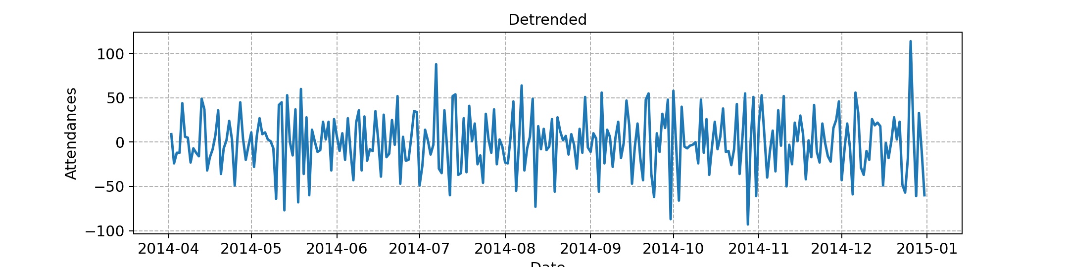
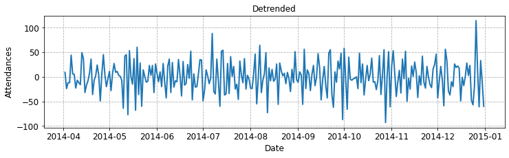
plot_detrended

For a given ED time series, this function generates and plots a differenced or detrended ED time series. The 1st difference is the difference between \(y_{t+1}\) and \(y_t\).

The output of the function should be a plot similar to the below. The function could return the fig and ax objects for a user.

detrended

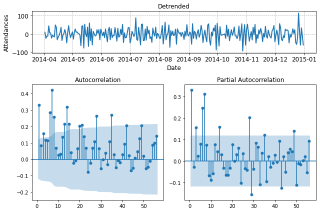
diagnostics_plot

For a given ED time series, the function will generate a plot similar to the below:

diag

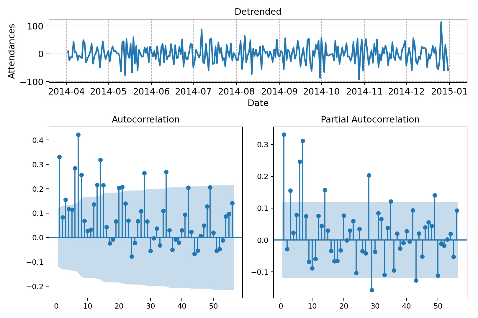
The figure consists of three axis objects. The first plots the detrended series. The second plot is the autocorrelation function (ACF): a measure of correlation of a variable with previous observations of itself. The third is the partial autocorrelation function (PACF): a measure of correlation of a variable with early observations of itself while controlling (regressing) for shorter lags. The good news is you can create ACF and PACF using two functions from statsmodels

#  import the functions
from statsmodels.graphics.tsaplots import plot_acf, plot_pacf

Task:

Code the plot_detrended and diagnostics_plot functions and add them to the ts_emergency/plotting/tsa module.

Hints:

diagnostics_plot is a good test of your matplotlib skills!
Try creating each plot indipendently first.
Note that the plot_acf and plot_pacf accepts a ax parameter. Can you use this parameter? to add the plot to the correct place?
There are various ways to answer this question. Consider using a gridspec.
Check out documentation for plot_acf and plot_pacf on the statsmodels docs. For example

# your package testing code here ...

# example solution testing package.
from ts_emergency.plotting.view import plot_single_ed
from ts_emergency.plotting.tsa import plot_detrended, diagnostic_plot
from ts_emergency.datasets import load_ed_ts

df = load_ed_ts()

fig, ax = plot_detrended(df, 'hosp_1')
#fig.savefig('im/detrended.jpg', dpi=180)

../../../_images/d4c2e3fb1ccf03c172ed56f9bd255b8bfa81875b10aa1fb3135b84fe20ec6524.png

fig, ax = diagnostic_plot(df, 'hosp_1')
#fig.savefig('im/diag.jpg', dpi=180)

../../../_images/ac04508ec1db11a90ce63957de45979391e35daaced97ffa3d5e6a7276d5e0d0.png

Example code for the tsa module#

'''
tsa - time series analysis module

plotting functions for time series analysis
'''

# standard imports
import matplotlib.pyplot as plt
import numpy as np
from statsmodels.graphics.tsaplots import plot_acf, plot_pacf

# cross package imports
from ts_emergency.plotting.view import plot_single_ed

def plot_detrended(wide_df, hosp_id, ax=None):
    '''
    Plot the first difference of the ED time series
    '''
    
    # create differenced dataframe
    diff_df = wide_df.diff(periods=1)
    
    fig, ax = plot_single_ed(diff_df, hosp_id, ax)
    ax.set_title('Detrended')
    
    return fig, ax
    

def diagnostic_plot(wide_df, hosp_id, figsize=(9, 6), maxlags=56, 
                    include_zero=False):
    '''
    Basic plot of diagnostics for ED time series.
    
    1. Detrended series
    2. ACF
    3. PACF
    
    Params:
    ------
    wide_df: pandas.Dataframe
        ED data in wide format
        
    hosp_id: str
        column name for hospital
        
    figsize: (int, int), optional (default=(9,6))
        size of figure
        
    maxlags: int, optional (default=56)
        The number of lags to include int the ACF and PACF
        
    include_zero: bool, optional (default=False)
        Include ACF and PACF of observation with itself in plot (=1.0)
    
    Returns:
    -------
    fig, np.ndarray
    ''' 
    fig = plt.figure(figsize=figsize, tight_layout=True)

    # add gridspec
    gs = fig.add_gridspec(3, 2)

    # detrended axis spans two columns
    ax1 = fig.add_subplot(gs[0, :])
    # acf axis spans 2 rows in column idx 0
    ax2 = fig.add_subplot(gs[1:,0])
    # pacf axis spans 2 rows in column idx 1
    ax3 = fig.add_subplot(gs[1:, 1])
    
    # plot detrended on axis 1
    _ = plot_detrended(wide_df, hosp_id, ax=ax1)

    # plot acf on axis 2
    _ = plot_acf(wide_df[hosp_id], lags=maxlags, ax=ax2, zero=include_zero)
    # plot pacf on axi
    _ = plot_pacf(wide_df[hosp_id], lags=maxlags, ax=ax3, zero=include_zero)
    
    axs = np.array([ax1, ax2, ax3])
    return fig, axs

    

Exercise 7:#

Task

Think about python programmes you have coded in the past. Can you think of how you would organise them as packages i.e. package name, submodules and example data? Choose a suitable example and draft an outline the structure of the package.

Python package exercise

Contents

Python package exercise#

Exercise 1#

Exercise 2:#

Exercise 3:#

Exercise 4:#

Exercise 5#

Exercise 6#

Example code for the tsa module#

Exercise 7:#